Build reference model for mouse testicular cell atlas
Compiled: November 06, 2023
Source:vignettes/model_mtca.Rmd
model_mtca.RmdIn this tutorial, we showed how to build a reference model for mouse testicular atlas. As germ cells undergo continuous development called spermatogenesis, we introduced consensus non-negative matrix factorization (cNMF) for feature selection rather than identifying cell markers via differential expression analysis usually adopted in the discrete cell clusters.
Download Reference Atlas
library(ProjectSVR)
library(Seurat)
library(tidyverse)
options(timeout = max(3600, getOption("timeout")))
`%notin%` <- Negate(`%in%`)
OUTPATH = "mTCA"
dir.create(OUTPATH)

get_label_pos <- function(data, emb = "tSNE", group.by="ClusterID") {
  new.data <- data[, c(paste(emb, 1:2, sep = "_"), group.by)]
  colnames(new.data) <- c("x","y","cluster")
  clusters <- names(table(new.data$cluster))
  new.pos <- lapply(clusters, function(i) {
    tmp.data = subset(new.data, cluster == i)
    data.frame(
      x = median(tmp.data$x),
      y = median(tmp.data$y),
      label = i)
  })
  do.call(rbind, new.pos)
}
if (!dir.exists("reference")) dir.create("reference")

download.file(url = "https://zenodo.org/record/8350746/files/mTCA.seurat.slim.qs",
              destfile = "reference/mTCA.seurat.slim.qs")
Feature Selection
Load reference data
data("pals")
seu.ref <- qs::qread("reference/mTCA.seurat.slim.qs")

data.plot <- FetchData(seu.ref, vars = c(paste0("UMAP_", 1:2), "Cell_type_symbol", "Cell_type_id"))

data.plot$Cell_type_id <- paste0("m", data.plot$Cell_type_id)
text.pos <- get_label_pos(data.plot, emb = "UMAP", group.by = "Cell_type_id")

ggplot(data.plot, aes(UMAP_1, UMAP_2, color = Cell_type_symbol), pt.size = .4) +
  geom_point(size = .1, alpha = .3) +
  scale_color_manual(values = pals$mtca) +
  ggtitle("Mouse testicular cell atlas") +
  geom_text(inherit.aes = F, data = text.pos,
            mapping = aes(x, y, label = label), size = 3) +
  guides(color = guide_legend(ncol = 2, override.aes = list(size = 4, alpha = 1))) +
  DimTheme()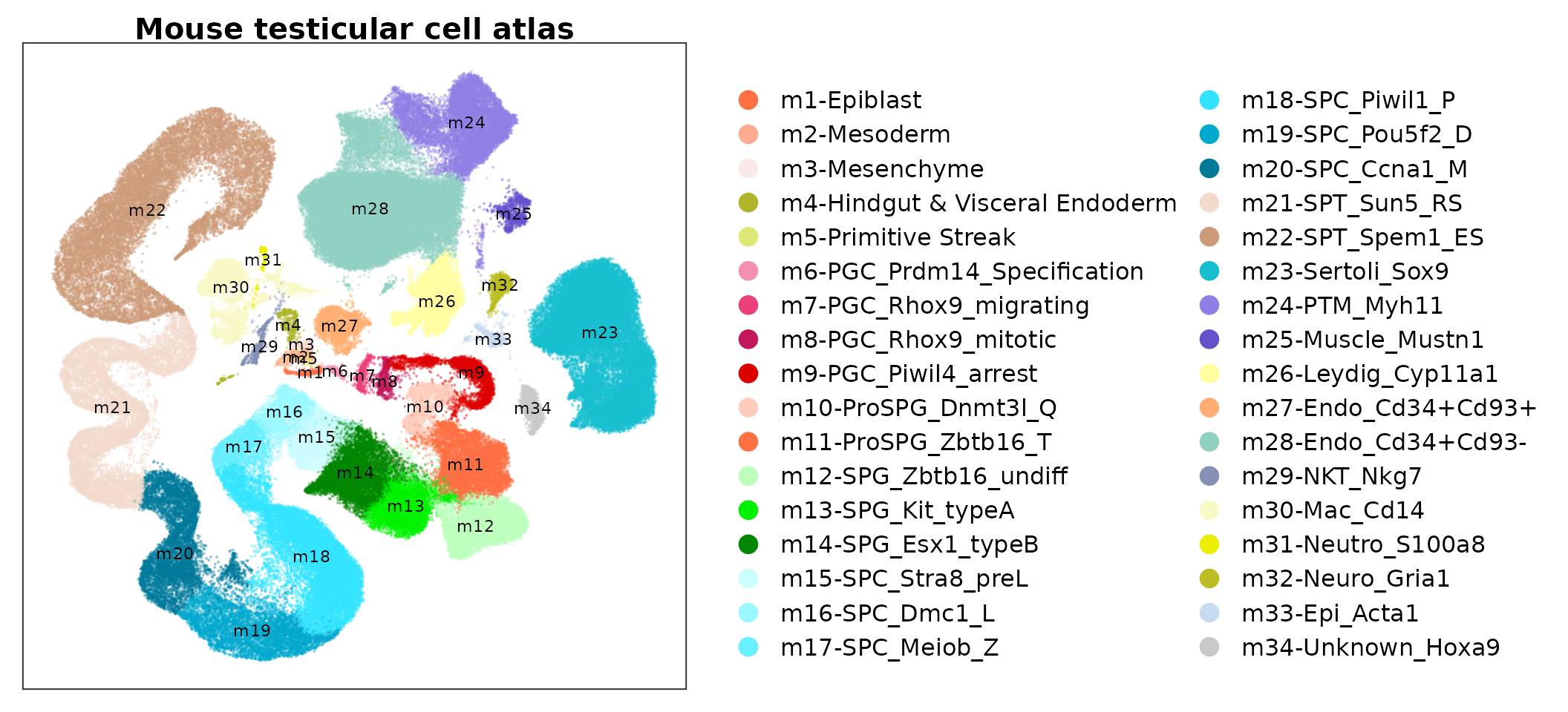
Make meta cells
Here, we introduce the cNMF methods for signature extraction.
To speed up the cNMF procedure, we utilize the metacell method that merges the adjacent cells in UMAP space into metacells.
## Grid the adjacent cells in the UMAP space.
emb.mat <- seu.ref[["umap"]]@cell.embeddings
gd <- EstimateKnnDensity(emb.mat = emb.mat)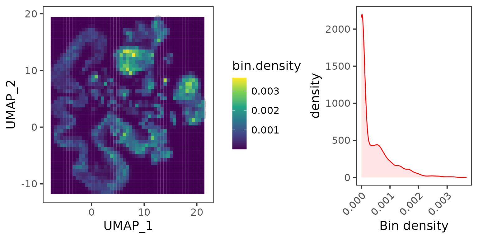
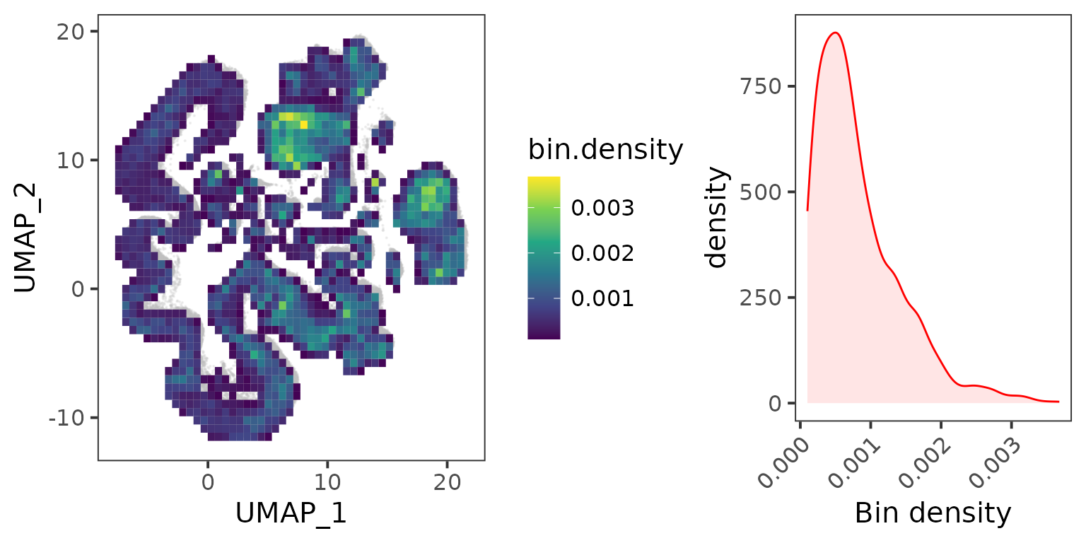
## Make meta cells
metacell.counts <- MergeCells(seu.ref[["RNA"]]@data, gd = gd, by = "mesh.points", cores = 10)
dim(metacell.counts)
## [1] 32285 3934Now we compress the 188,862 cells into 3934 meta cells.
## The genes expressed in at least 20 cells were kept.
expr.in.cells <- Matrix::rowSums(metacell.counts > 0)
metacell.counts <- metacell.counts[expr.in.cells >= 20, ]

## Drop mitochondrial genes
is.mito <- grepl("^mt-", rownames(metacell.counts))
metacell.counts <- metacell.counts[!is.mito, ]

## Transfer the Seurat format into h5ad file.
seu.mc <- CreateSeuratObject(counts = metacell.counts)
sceasy::convertFormat(seu.mc, from = "seurat", to = "anndata", main_layer = "counts",
                      outFile = file.path(OUTPATH, "mTCA.metacells.h5ad"))
## Save HVGs: generated in data integration step
writeLines(seu.ref[["RNA"]]@var.features, file.path(OUTPATH, "mTCA.metacells.hvgs.txt"))

rm(seu.mc)
rm(metacell.counts)
gc()
Run cNMF
FindOptimalK(counts.fn = file.path(OUTPATH, "mTCA.metacells.h5ad"),
             run.name = "K20_K100_by5",
             components = seq(20,100,5),
             genes.fn = file.path(OUTPATH, "mTCA.metacells.hvgs.txt"),
             out.path = OUTPATH,
             n.iter = 20,
             cores = 20)
This will generate a deagnostic plot for the K selection under
mTCA/K20_K100_by5/K20_K100_by5.k_selection.png.
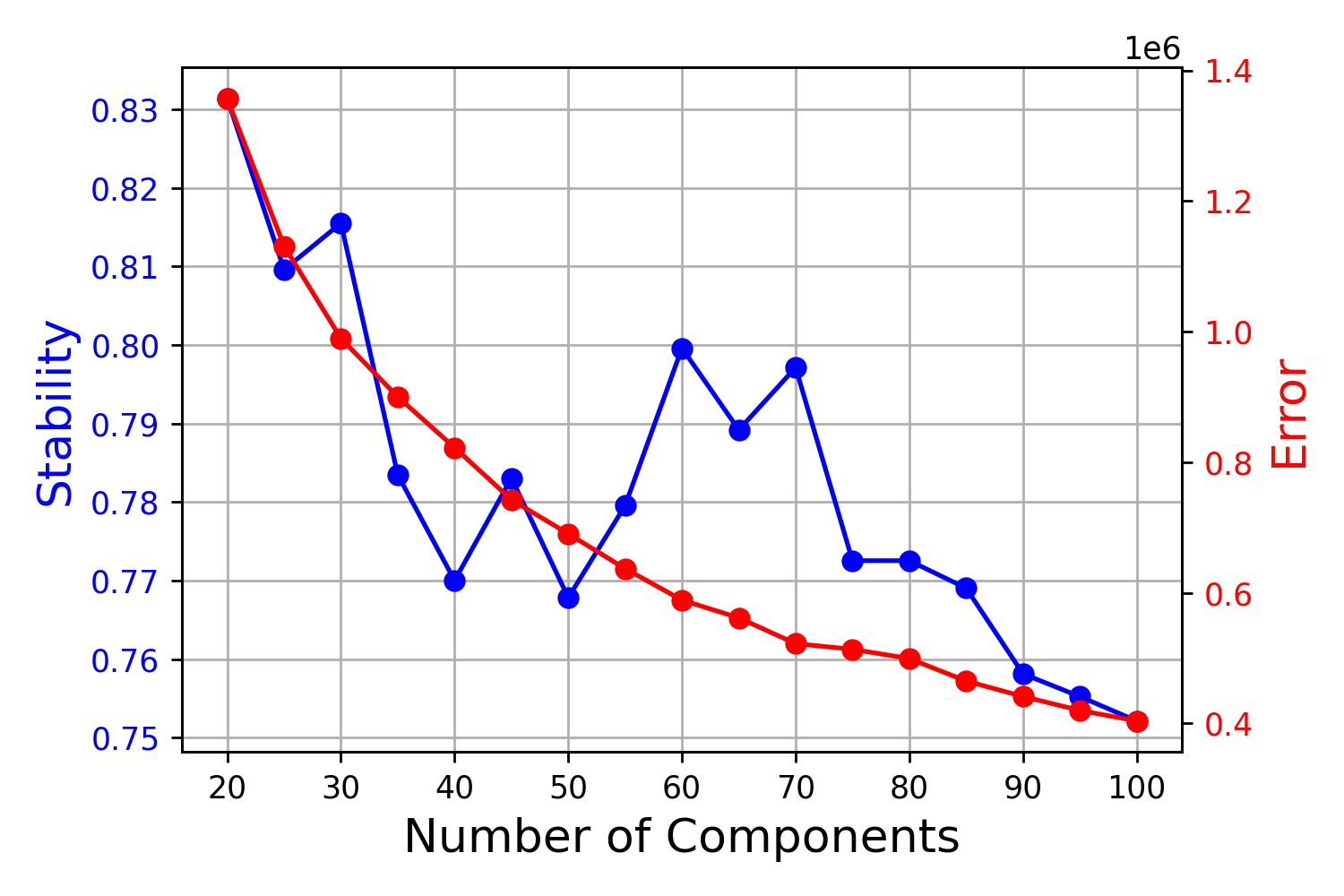
The solution of K = 70 makes the decomposition the less reconstruction error without the loss of solution robustness.
Transfer raw count matrix to gene set score matrix
Here, we try the AUCell method for calculating signature scores.
top.genes <- read.table(file.path(OUTPATH, "K70/top100_genes.k_70.dt_0_2.txt"), header = T)
names(top.genes) <- paste0("feature.", 1:length(top.genes))
seu.ref <- ComputeModuleScore(seu.ref, gene.sets = top.genes, method = "AUCell", cores = 5)
# The signature score matrix is stored in 'SignatureScore' assay
Assays(seu.ref)
DefaultAssay(seu.ref) <- "SignatureScore"

gss.mat <- FetchData(seu.ref, vars = rownames(seu.ref))
saveRDS(gss.mat, file.path(OUTPATH, "mTCA.AUCell.rds"))
gss.mat <- readRDS(file.path(OUTPATH, "mTCA.AUCell.rds"))
data.plot <- FetchData(seu.ref, vars = paste0("UMAP_", 1:2) )
data.plot <- cbind(gss.mat, data.plot)

data.plot <- data.plot %>%
  pivot_longer(cols = 1:70, names_to = "component", values_to = "score")

data.plot %>%
  group_split(component) %>%
  map(
    ~ggplot(., aes(UMAP_1, UMAP_2, color = score)) +
      geom_point(size = .5) +
      scale_color_viridis_c() +
      facet_grid(~ component, labeller = function(x) label_value(x, multi_line = FALSE)) +
      theme_bw(base_size = 15)
  ) %>%
  cowplot::plot_grid(plotlist = ., align = 'hv', ncol = 7)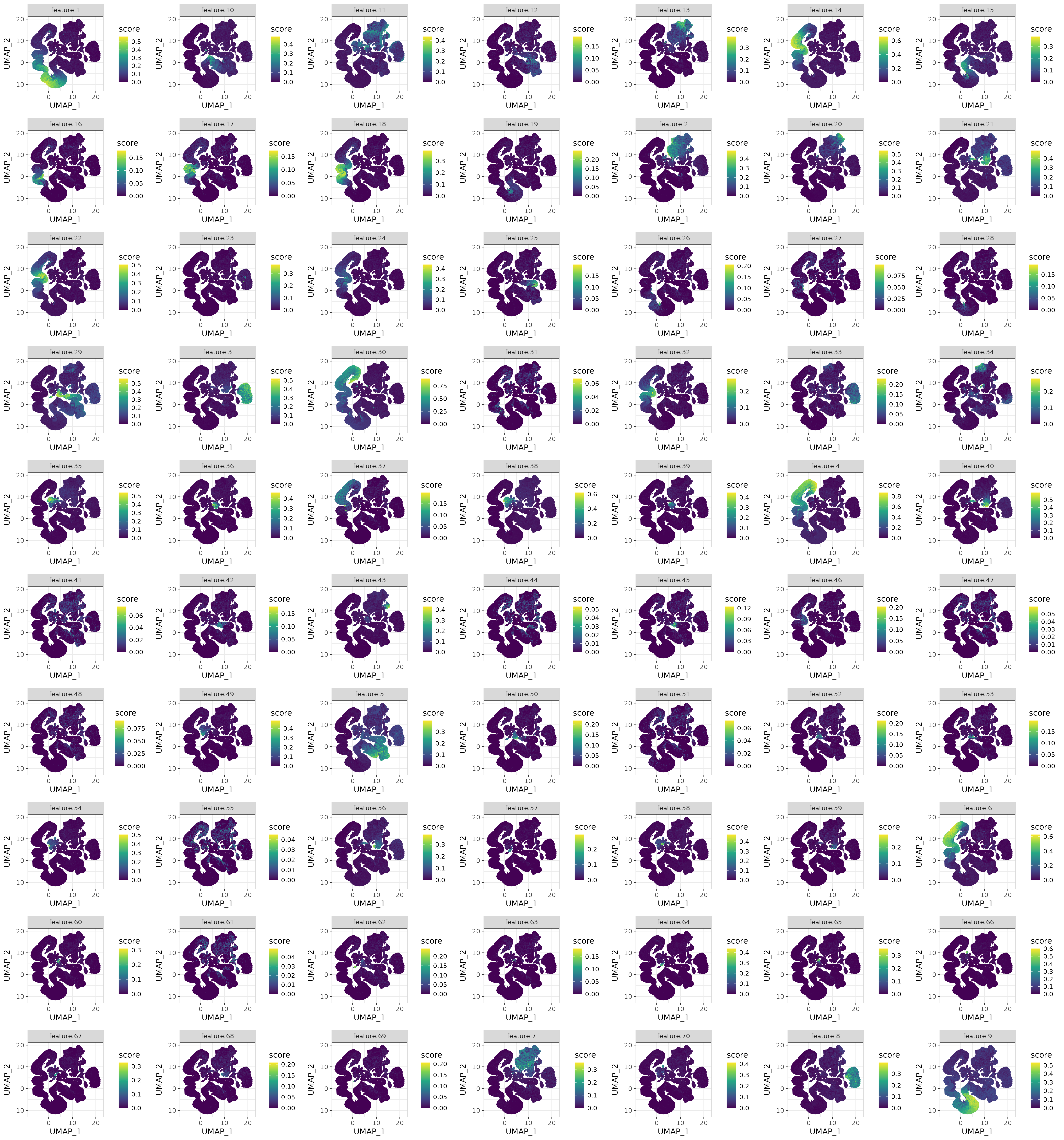
Build Reference Model
Training reference model
# Training model
gss.mat <- readRDS(file.path(OUTPATH, "mTCA.AUCell.rds"))
embeddings.df <- FetchData(seu.ref, vars = paste0("UMAP_", 1:2))
batch.size = 8000 # number of subsampled cells for each SVR model
n.models = 20     # number of SVR models trained
umap.model <- FitEnsembleSVM(feature.mat = gss.mat,
                             emb.mat = embeddings.df,
                             batch.size = batch.size,
                             n.models = n.models,
                             cores = 10)
Create reference object
meta.data: cell meta data (embeddings & cell type information)
gss.method: method used in
ComputeModuleScore()[optional] colors: for plots
[optional] text.pos: text annotation on the reference plots
meta.data <- FetchData(seu.ref, vars = c(paste0("UMAP_", 1:2), "Cell_type_symbol"))
colnames(meta.data)[3] <- c("cell_type")

colors <- pals$mtca

reference <- CreateReference(umap.model = umap.model,
                             gene.sets = top.genes,
                             meta.data = meta.data,
                             gss.method = "AUCell",
                             colors = colors,
                             text.pos = text.pos)

if (!dir.exists("models")) dir.create("models")
saveRDS(reference, "models/model.mTCA.rds")
Session Info
## R version 4.1.2 (2021-11-01)
## Platform: x86_64-pc-linux-gnu (64-bit)
## Running under: Ubuntu 22.04.2 LTS
##
## Matrix products: default
## BLAS:   /usr/lib/x86_64-linux-gnu/blas/libblas.so.3.10.0
## LAPACK: /usr/lib/x86_64-linux-gnu/lapack/liblapack.so.3.10.0
##
## locale:
##  [1] LC_CTYPE=C.UTF-8       LC_NUMERIC=C           LC_TIME=C.UTF-8
##  [4] LC_COLLATE=C.UTF-8     LC_MONETARY=C.UTF-8    LC_MESSAGES=C.UTF-8
##  [7] LC_PAPER=C.UTF-8       LC_NAME=C              LC_ADDRESS=C
## [10] LC_TELEPHONE=C         LC_MEASUREMENT=C.UTF-8 LC_IDENTIFICATION=C
##
## attached base packages:
## [1] stats     graphics  grDevices utils     datasets  methods   base
##
## other attached packages:
##  [1] lubridate_1.9.2    forcats_1.0.0      stringr_1.5.0      dplyr_1.1.3
##  [5] purrr_1.0.2        readr_2.1.4        tidyr_1.3.0        tibble_3.2.1
##  [9] ggplot2_3.4.3      tidyverse_2.0.0    SeuratObject_4.1.3 Seurat_4.3.0.1
## [13] ProjectSVR_0.2.0
##
## loaded via a namespace (and not attached):
##   [1] utf8_1.2.3             spatstat.explore_3.2-3 reticulate_1.31
##   [4] tidyselect_1.2.0       mlr3learners_0.5.6     htmlwidgets_1.6.2
##   [7] grid_4.1.2             Rtsne_0.16             mlr3misc_0.12.0
##  [10] munsell_0.5.0          codetools_0.2-18       bbotk_0.7.2
##  [13] ragg_1.2.5             ica_1.0-3              future_1.33.0
##  [16] miniUI_0.1.1.1         mlr3verse_0.2.8        withr_2.5.0
##  [19] spatstat.random_3.1-6  colorspace_2.1-0       progressr_0.14.0
##  [22] highr_0.10             knitr_1.43             uuid_1.1-1
##  [25] rstudioapi_0.15.0      stats4_4.1.2           ROCR_1.0-11
##  [28] robustbase_0.99-0      tensor_1.5             listenv_0.9.0
##  [31] labeling_0.4.3         mlr3tuning_0.19.0      polyclip_1.10-4
##  [34] lgr_0.4.4              farver_2.1.1           rprojroot_2.0.3
##  [37] parallelly_1.36.0      vctrs_0.6.3            generics_0.1.3
##  [40] xfun_0.40              timechange_0.2.0       diptest_0.76-0
##  [43] R6_2.5.1               doParallel_1.0.17      clue_0.3-64
##  [46] flexmix_2.3-19         spatstat.utils_3.0-3   cachem_1.0.8
##  [49] promises_1.2.1         scales_1.2.1           nnet_7.3-17
##  [52] gtable_0.3.4           globals_0.16.2         goftest_1.2-3
##  [55] mlr3hyperband_0.4.5    mlr3mbo_0.2.1          rlang_1.1.1
##  [58] systemfonts_1.0.4      GlobalOptions_0.1.2    splines_4.1.2
##  [61] lazyeval_0.2.2         paradox_0.11.1         spatstat.geom_3.2-5
##  [64] checkmate_2.2.0        yaml_2.3.7             reshape2_1.4.4
##  [67] abind_1.4-5            mlr3_0.16.1            backports_1.4.1
##  [70] httpuv_1.6.11          tools_4.1.2            ellipsis_0.3.2
##  [73] jquerylib_0.1.4        RColorBrewer_1.1-3     BiocGenerics_0.40.0
##  [76] ggridges_0.5.4         Rcpp_1.0.11            plyr_1.8.8
##  [79] deldir_1.0-9           pbapply_1.7-2          GetoptLong_1.0.5
##  [82] cowplot_1.1.1          S4Vectors_0.32.4       zoo_1.8-12
##  [85] ggrepel_0.9.3          cluster_2.1.2          fs_1.6.3
##  [88] magrittr_2.0.3         data.table_1.14.8      scattermore_1.2
##  [91] circlize_0.4.15        lmtest_0.9-40          RANN_2.6.1
##  [94] fitdistrplus_1.1-11    matrixStats_1.0.0      stringfish_0.15.8
##  [97] qs_0.25.5              hms_1.1.3              patchwork_1.1.3
## [100] mime_0.12              evaluate_0.21          xtable_1.8-4
## [103] mclust_6.0.0           IRanges_2.28.0         gridExtra_2.3
## [106] shape_1.4.6            compiler_4.1.2         mlr3cluster_0.1.8
## [109] KernSmooth_2.23-20     crayon_1.5.2           htmltools_0.5.6
## [112] tzdb_0.4.0             later_1.3.1            RcppParallel_5.1.7
## [115] RApiSerialize_0.1.2    ComplexHeatmap_2.10.0  MASS_7.3-55
## [118] fpc_2.2-10             mlr3data_0.7.0         Matrix_1.6-1
## [121] cli_3.6.1              parallel_4.1.2         igraph_1.5.1
## [124] pkgconfig_2.0.3        pkgdown_2.0.7          sp_2.0-0
## [127] plotly_4.10.2          spatstat.sparse_3.0-2  foreach_1.5.2
## [130] bslib_0.5.1            mlr3fselect_0.11.0     digest_0.6.33
## [133] sctransform_0.3.5      RcppAnnoy_0.0.21       mlr3filters_0.7.1
## [136] spatstat.data_3.0-1    rmarkdown_2.24         leiden_0.4.3
## [139] uwot_0.1.16            kernlab_0.9-32         shiny_1.7.5
## [142] modeltools_0.2-23      rjson_0.2.21           nlme_3.1-155
## [145] lifecycle_1.0.3        jsonlite_1.8.7         mlr3tuningspaces_0.4.0
## [148] desc_1.4.2             viridisLite_0.4.2      fansi_1.0.4
## [151] pillar_1.9.0           lattice_0.20-45        fastmap_1.1.1
## [154] httr_1.4.7             DEoptimR_1.1-2         survival_3.2-13
## [157] glue_1.6.2             mlr3viz_0.6.1          png_0.1-8
## [160] prabclus_2.3-2         iterators_1.0.14       spacefillr_0.3.2
## [163] class_7.3-20           stringi_1.7.12         sass_0.4.7
## [166] mlr3pipelines_0.5.0-1  palmerpenguins_0.1.1   textshaping_0.3.6
## [169] memoise_2.0.1          irlba_2.3.5.1          future.apply_1.11.0