Accurate identification of the tumor-infiltrated T cell heterogeneity in cancer immunology study
Compiled: November 06, 2023
Source:vignettes/mapQuery_ICB_BRCA.Rmd
mapQuery_ICB_BRCA.RmdIn recent years, single-cell RNA-sequencing (scRNA-seq) enabled unbiased exploration of T cell diversity in health, disease and response to therapies at an unprecedented scale and resolution. However, a comprehensive definition of T cell “reference” subtypes remains elusive 1.
Several groups try to integrate T cells in the tumor micro-environment (TME) across different cancer types to build a pan-cancer T cell landscape. For example, Zheng et al. depicted a pan-cancer landscape of T cell heterogeneity in the TME and established a baseline reference for future scRNA-seq studies associated with cancer treatments 2.
In this tutorial, we demonstrate the process of projecting query T cells onto the pan-cancer T cell landscape (PTCL) to interpret the disparities in CD8 T cell heterogeneity between responsive and non-responsive patients with breast cancer who have undergone immune checkpoint blockade (ICB) therapy 3. This will be done using ProjectSVR.
Download Related Dataset
library(Seurat)
library(ProjectSVR)
library(tidyverse)
options(timeout = max(3600, getOption("timeout")))
# reference model
if (!dir.exists("models")) dir.create("models")
download.file(url = "https://zenodo.org/record/8350732/files/model.Zheng2021.CD8Tcell.rds",
              destfile = "models/model.Zheng2021.CD8Tcell.rds")
# query data
if (!dir.exists("query")) dir.create("query")
download.file(url = "https://zenodo.org/record/8350748/files/ICB_BRCA.1864-counts_cd8tcell_cohort1.seurat.rds",
              destfile = "query/ICB_BRCA.1864-counts_cd8tcell_cohort1.seurat.rds")
Map Query to Reference
Reference mapping
reference <- readRDS("models/model.Zheng2021.CD8Tcell.rds")
seu.q <- readRDS("query/ICB_BRCA.1864-counts_cd8tcell_cohort1.seurat.rds")

annotations <- c(
  "E" = "Responders",
  "n/a" = "n/a",
  "NE" = "Non-Responders"
)
seu.q$group <- annotations[seu.q$expansion]

seu.q <- ProjectSVR::MapQuery(seu.q, reference = reference,
                              add.map.qual = T, ncores = 10)

p1 <- DimPlot(seu.q, reduction = "ref.umap", group.by = "patient_id")
p2 <- DimPlot(seu.q, reduction = "ref.umap", group.by = "cellSubType",
              label = T) + ggsci::scale_color_d3("category20")
p1 + p2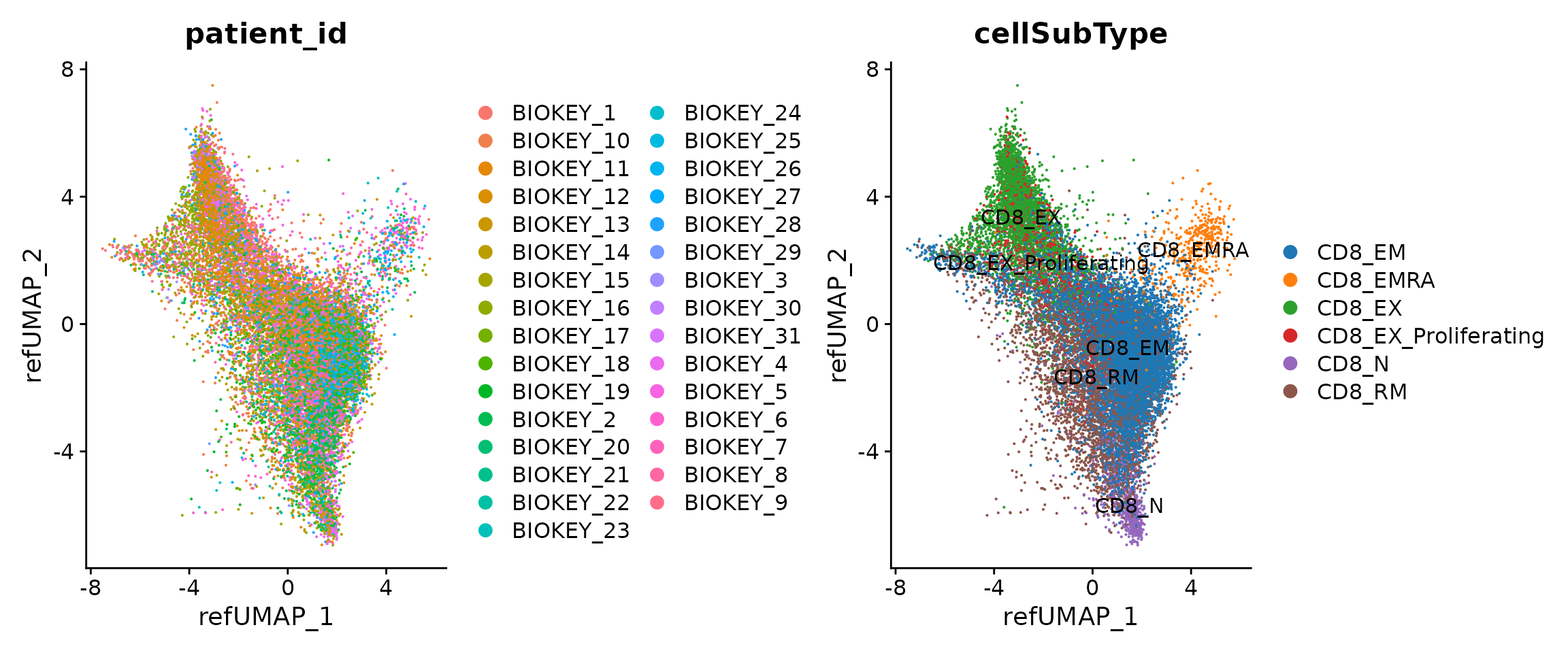
Maping quality
Determine the threshold to distinguish the good and bad projections.
QC plot for the reference mapping.
## cutoff by adjusted p value
MapQCPlot(seu.q, p.adj.cutoff = 1e-3)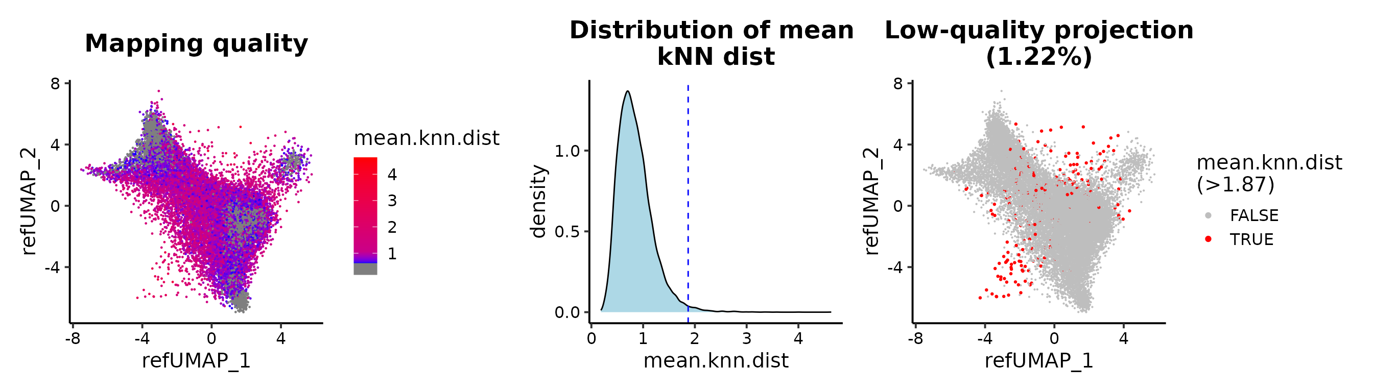
## or mean.knn.dist
MapQCPlot(seu.q, map.q.cutoff = 1.6)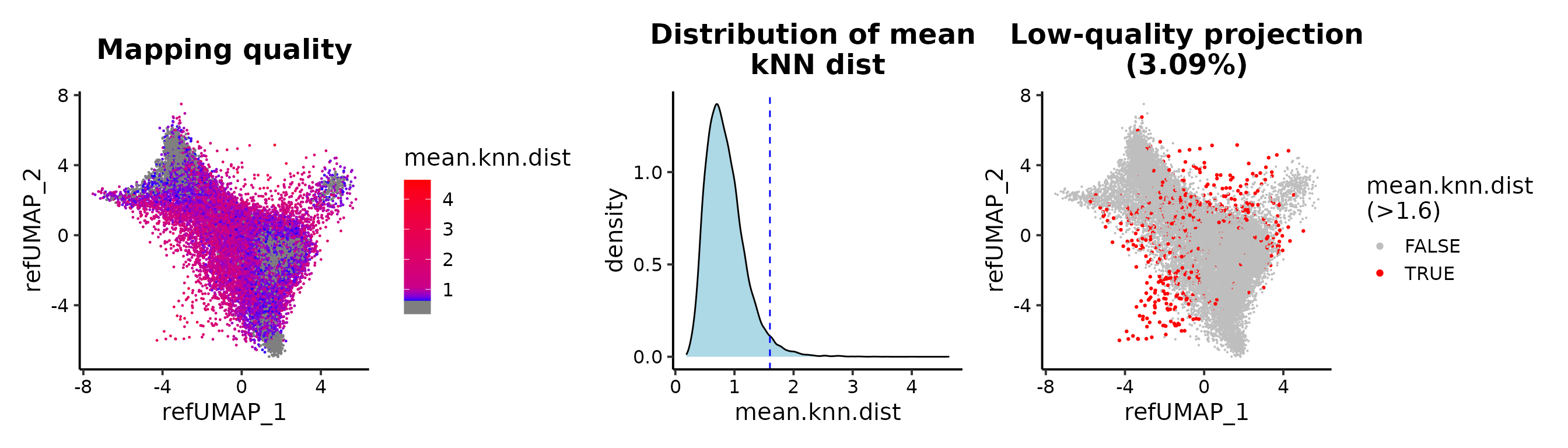
Visualize the projected query cells onto the reference atlas.
PlotProjection(seu.q, reference, split.by = "cellSubType", ref.color.by = "cluster.name",
               ref.size = .5, ref.alpha = .3, query.size = 1, query.alpha = .5, n.row = 2)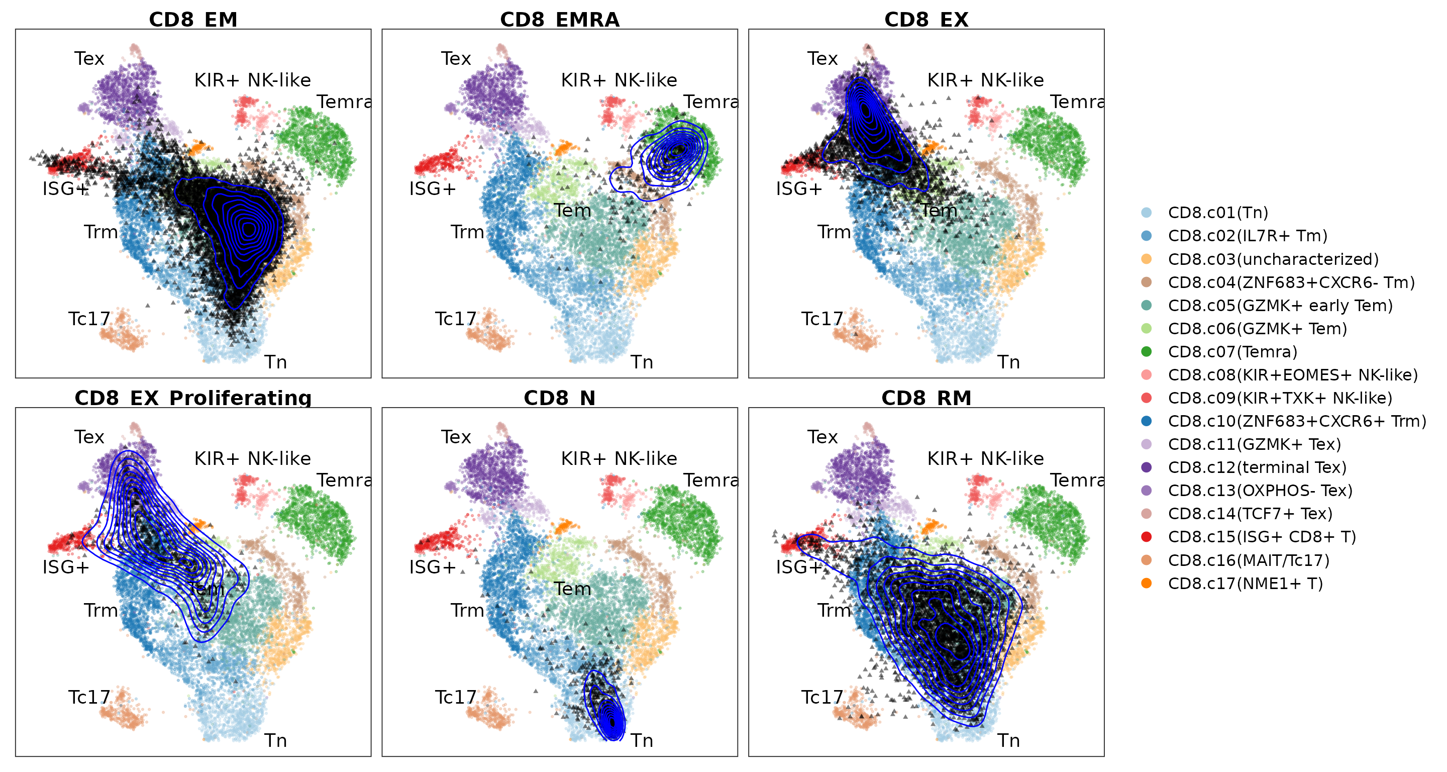
Label transfer
seu.q <- ProjectSVR::LabelTransfer(seu.q, reference, ref.label.col = "cluster.name")Differential cell population
seu.q <- subset(seu.q, group != "n/a" & timepoint == "Pre")
seu.q <- subset(seu.q, mean.knn.dist < 1.6)
seu.q$group <- factor(seu.q$group)

PlotProjection(seu.q, reference, split.by = "group", ref.color.by = "cluster.name",
               ref.size = .5, ref.alpha = .3, query.size = 1, query.alpha = .5, n.row = 1)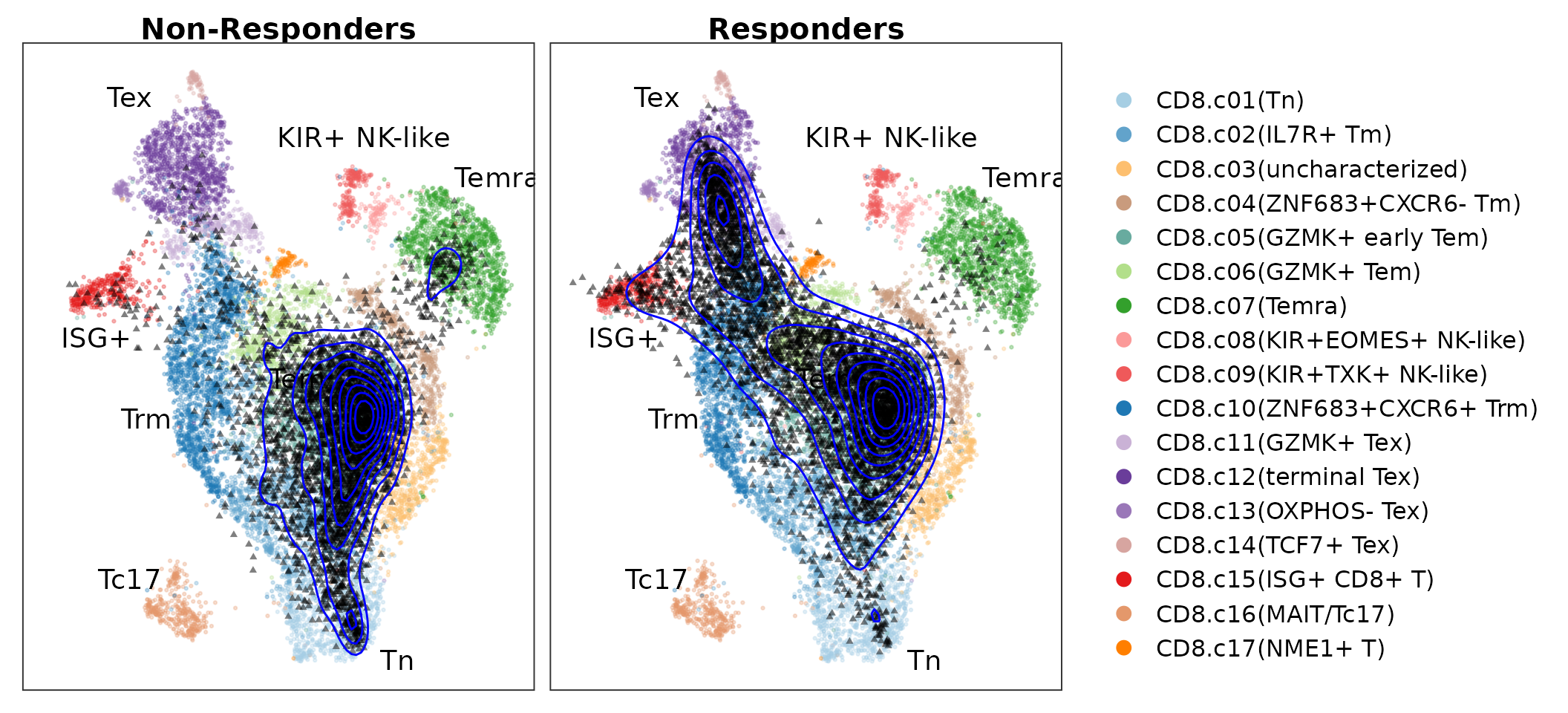
Alluvia plot
AlluviaPlot(seu.q@meta.data, by = "group", fill = "knn.pred.celltype",
            colors = reference$ref.cellmeta$colors,
            bar.width = .5)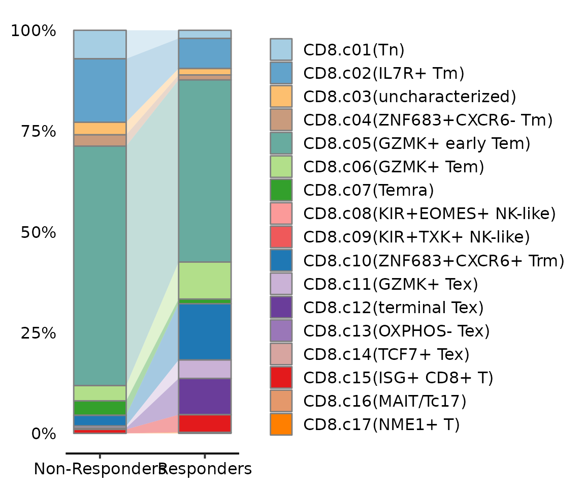
Preference analysis
GroupPreferencePlot(seu.q@meta.data, group.by = "group",
                    preference.on = "knn.pred.celltype",
                    column_names_rot = 0, column_names_centered = TRUE)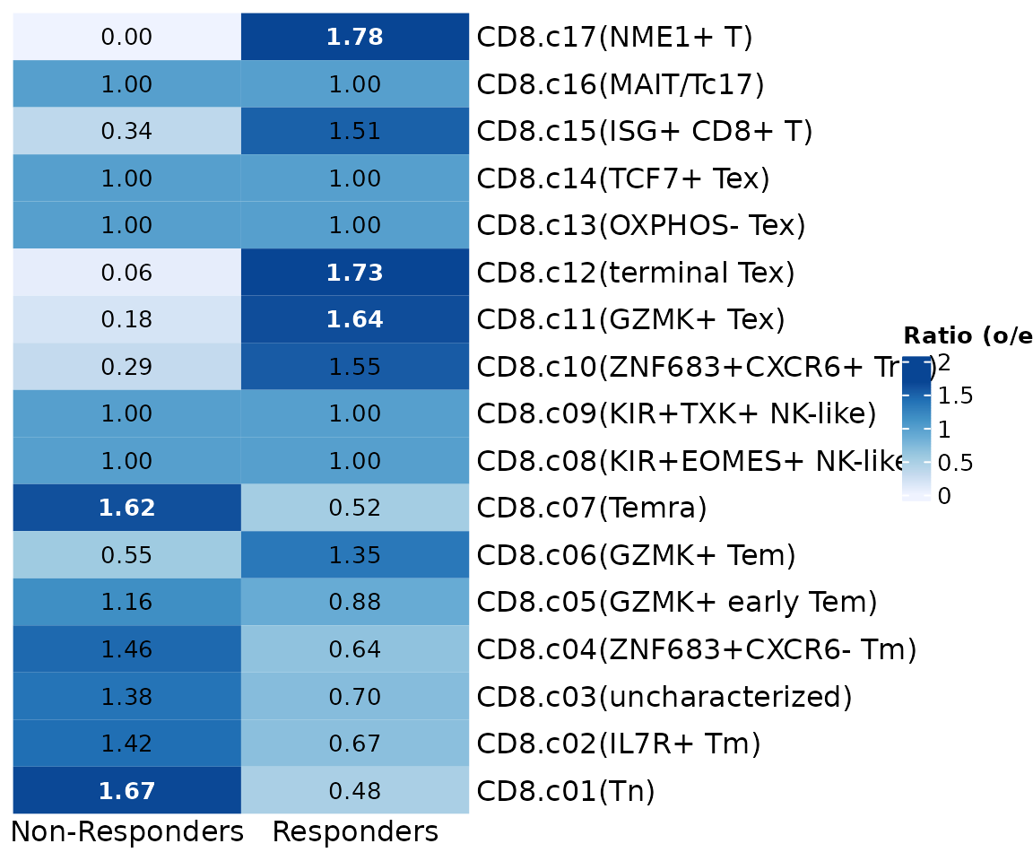
If seu.q$knn.pred.celltype was not a factor, then rows
were ordered by o/e value.
meta.data <- seu.q@meta.data
meta.data$knn.pred.celltype <- as.character(meta.data$knn.pred.celltype)
GroupPreferencePlot(meta.data, group.by = "group",
                    preference.on = "knn.pred.celltype",
                    column_names_rot = 0, column_names_centered = TRUE)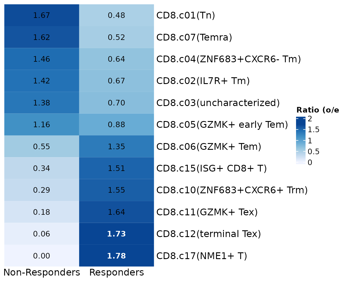
Wilcoxon test
da.test <- AbundanceTest(cellmeta = seu.q@meta.data,
                         celltype.col = "knn.pred.celltype",
                         sample.col = "patient_id",
                         group.col = "group")

## Volcano plot
VolcanoPlot(da.test, xlab = "log2(R / NR)", ylab = "Frequency",
            colors = reference$ref.cellmeta$colors)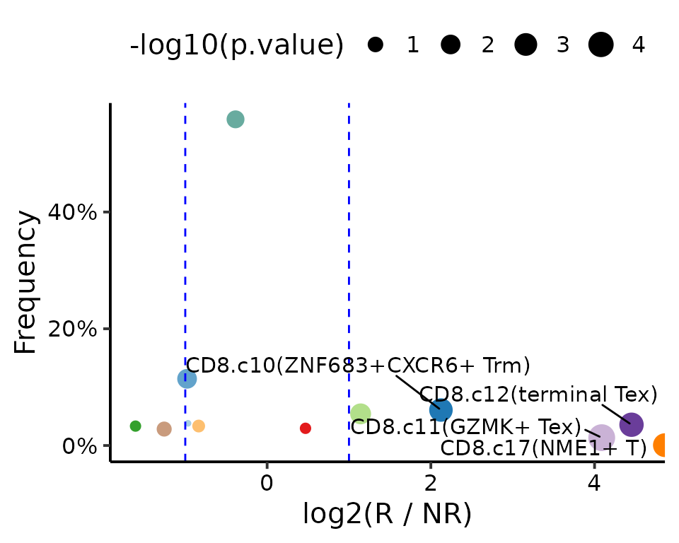
Focus on the detailed information via BoxPlot().
## Box plot
BoxPlot(cellmeta = seu.q@meta.data, celltype.col = "knn.pred.celltype",
        sample.col = "patient_id", group.col = "group",
        celltypes.show = c("CD8.c12(terminal Tex)", "CD8.c11(GZMK+ Tex)"),
        legend.ncol = 2) +
  scale_x_discrete(labels = c("NR", "R"))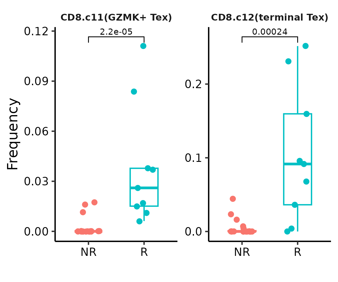
Session Info
## R version 4.1.2 (2021-11-01)
## Platform: x86_64-pc-linux-gnu (64-bit)
## Running under: Ubuntu 22.04.2 LTS
##
## Matrix products: default
## BLAS:   /usr/lib/x86_64-linux-gnu/blas/libblas.so.3.10.0
## LAPACK: /usr/lib/x86_64-linux-gnu/lapack/liblapack.so.3.10.0
##
## locale:
##  [1] LC_CTYPE=C.UTF-8       LC_NUMERIC=C           LC_TIME=C.UTF-8
##  [4] LC_COLLATE=C.UTF-8     LC_MONETARY=C.UTF-8    LC_MESSAGES=C.UTF-8
##  [7] LC_PAPER=C.UTF-8       LC_NAME=C              LC_ADDRESS=C
## [10] LC_TELEPHONE=C         LC_MEASUREMENT=C.UTF-8 LC_IDENTIFICATION=C
##
## attached base packages:
## [1] stats     graphics  grDevices utils     datasets  methods   base
##
## other attached packages:
##  [1] lubridate_1.9.2    forcats_1.0.0      stringr_1.5.0      dplyr_1.1.3
##  [5] purrr_1.0.2        readr_2.1.4        tidyr_1.3.0        tibble_3.2.1
##  [9] ggplot2_3.4.3      tidyverse_2.0.0    ProjectSVR_0.2.0   SeuratObject_4.1.3
## [13] Seurat_4.3.0.1
##
## loaded via a namespace (and not attached):
##   [1] utf8_1.2.3             spatstat.explore_3.2-3 reticulate_1.31
##   [4] tidyselect_1.2.0       mlr3learners_0.5.6     htmlwidgets_1.6.2
##   [7] BiocParallel_1.28.3    grid_4.1.2             Rtsne_0.16
##  [10] mlr3misc_0.12.0        munsell_0.5.0          codetools_0.2-18
##  [13] bbotk_0.7.2            ragg_1.2.5             ica_1.0-3
##  [16] future_1.33.0          miniUI_0.1.1.1         mlr3verse_0.2.8
##  [19] withr_2.5.0            spatstat.random_3.1-6  colorspace_2.1-0
##  [22] progressr_0.14.0       highr_0.10             knitr_1.43
##  [25] uuid_1.1-1             rstudioapi_0.15.0      stats4_4.1.2
##  [28] ROCR_1.0-11            robustbase_0.99-0      ggsignif_0.6.4
##  [31] tensor_1.5             listenv_0.9.0          labeling_0.4.3
##  [34] mlr3tuning_0.19.0      lgr_0.4.4              polyclip_1.10-4
##  [37] farver_2.1.1           rprojroot_2.0.3        parallelly_1.36.0
##  [40] vctrs_0.6.3            generics_0.1.3         xfun_0.40
##  [43] timechange_0.2.0       diptest_0.76-0         R6_2.5.1
##  [46] doParallel_1.0.17      clue_0.3-64            isoband_0.2.7
##  [49] flexmix_2.3-19         spatstat.utils_3.0-3   cachem_1.0.8
##  [52] promises_1.2.1         scales_1.2.1           nnet_7.3-17
##  [55] gtable_0.3.4           globals_0.16.2         mlr3hyperband_0.4.5
##  [58] goftest_1.2-3          mlr3mbo_0.2.1          rlang_1.1.1
##  [61] systemfonts_1.0.4      GlobalOptions_0.1.2    splines_4.1.2
##  [64] lazyeval_0.2.2         paradox_0.11.1         spatstat.geom_3.2-5
##  [67] checkmate_2.2.0        yaml_2.3.7             reshape2_1.4.4
##  [70] abind_1.4-5            mlr3_0.16.1            backports_1.4.1
##  [73] httpuv_1.6.11          tools_4.1.2            ellipsis_0.3.2
##  [76] jquerylib_0.1.4        RColorBrewer_1.1-3     BiocGenerics_0.40.0
##  [79] ggridges_0.5.4         Rcpp_1.0.11            plyr_1.8.8
##  [82] deldir_1.0-9           pbapply_1.7-2          GetoptLong_1.0.5
##  [85] cowplot_1.1.1          S4Vectors_0.32.4       zoo_1.8-12
##  [88] ggrepel_0.9.3          cluster_2.1.2          here_1.0.1
##  [91] fs_1.6.3               magrittr_2.0.3         data.table_1.14.8
##  [94] scattermore_1.2        circlize_0.4.15        lmtest_0.9-40
##  [97] RANN_2.6.1             fitdistrplus_1.1-11    matrixStats_1.0.0
## [100] hms_1.1.3              patchwork_1.1.3        mime_0.12
## [103] evaluate_0.21          xtable_1.8-4           mclust_6.0.0
## [106] IRanges_2.28.0         gridExtra_2.3          shape_1.4.6
## [109] UCell_1.3.1            compiler_4.1.2         mlr3cluster_0.1.8
## [112] KernSmooth_2.23-20     crayon_1.5.2           htmltools_0.5.6
## [115] tzdb_0.4.0             later_1.3.1            ComplexHeatmap_2.10.0
## [118] rappdirs_0.3.3         MASS_7.3-55            fpc_2.2-10
## [121] mlr3data_0.7.0         Matrix_1.6-1           cli_3.6.1
## [124] parallel_4.1.2         igraph_1.5.1           pkgconfig_2.0.3
## [127] pkgdown_2.0.7          sp_2.0-0               plotly_4.10.2
## [130] spatstat.sparse_3.0-2  foreach_1.5.2          bslib_0.5.1
## [133] mlr3fselect_0.11.0     digest_0.6.33          sctransform_0.3.5
## [136] RcppAnnoy_0.0.21       mlr3filters_0.7.1      spatstat.data_3.0-1
## [139] rmarkdown_2.24         leiden_0.4.3           uwot_0.1.16
## [142] kernlab_0.9-32         shiny_1.7.5            modeltools_0.2-23
## [145] rjson_0.2.21           lifecycle_1.0.3        nlme_3.1-155
## [148] jsonlite_1.8.7         mlr3tuningspaces_0.4.0 desc_1.4.2
## [151] viridisLite_0.4.2      fansi_1.0.4            pillar_1.9.0
## [154] ggsci_3.0.0            lattice_0.20-45        fastmap_1.1.1
## [157] httr_1.4.7             DEoptimR_1.1-2         survival_3.2-13
## [160] glue_1.6.2             mlr3viz_0.6.1          png_0.1-8
## [163] prabclus_2.3-2         iterators_1.0.14       spacefillr_0.3.2
## [166] class_7.3-20           stringi_1.7.12         sass_0.4.7
## [169] mlr3pipelines_0.5.0-1  palmerpenguins_0.1.1   textshaping_0.3.6
## [172] memoise_2.0.1          irlba_2.3.5.1          future.apply_1.11.0